One of the most important building blocks of computer graphics is interpolation: estimating intermediate values from known ones. Let’s explore a few applications using iKe, a frontend for the oK interpreter which augments it with simple drawing primitives. If you’re unfamiliar with iKe, take a glance at the manual or the tutorial article I wrote for Vector.
Given a sequence of color “stops”, we might wish to form a palette which blends from each to the next. Since iKe uses CSS color formats, it would be useful to start by defining some functions for converting hex color strings like "#C0FFEE" into unpacked Red-Green-Blue vectors like 192 255 238 and back again.
We can use a lookup table and ? (“find”) to get a sequence of more sensible hex digits from a string:
  hex: "0123456789ABCDEF"
"0123456789ABCDEF"

  1_"#C0FFEE"
"C0FFEE"

  0N 2#1_"#C0FFEE"
("C0"
 "FF"
 "EE")

  hex?0N 2#1_"#C0FFEE"
(12 0
 15 15
 14 14)
And then the verbs n\l and n/l (“decode” and “encode”) to translate between base-16 and base-10:
  16/'hex?0N 2#1_"#C0FFEE"
192 255 238

  16 16\'192 255 238
(12 0
 15 15
 14 14)
To linearly interpolate (sometimes given as the slang “lerp”), we scale the difference between each channel by a control value, here x, which will be varied within [0,1]. I’ll refer to this value as the tween.
  c: (226 188 51;232 122 15)
(226 188 51
 232 122 15)

  {{_y+x*z-y}[x]/c}'0 .25 .5 1
(226 188 51
 227 171 42
 229 155 33
 232 122 15)
Most of the complexity of building gradients lies in potential fencepost errors: we must make sure that the final gradient begins and ends exactly on our first and last color stop, and that we produce an interpolated palette with the right number of steps.
  stops: ("#E2BC33";"#E87A0F";"#FFFFFF";"#227EB6";"#2B7D2D")
("#E2BC33"
 "#E87A0F"
 "#FFFFFF"
 "#227EB6"
 "#2B7D2D")

  / inclusive [0,1] range
  {(!y)%y-1}[stops;10]
0 0.1111 0.2222 0.3333 0.4444 0.5556 0.6667 0.7778 0.8889 1

  / make sure we have the right number of steps
  {#(!y)%y-1}[stops;10]
10

  / steps scaled to line up with input palette
  {((#x)-1)*(!y)%y-1}[stops;10]
0 0.4444 0.8889 1.3333 1.7778 2.2222 2.6667 3.1111 3.5556 4

  / the tween for each interval
  {1!((#x)-1)*(!y)%y-1}[stops;10]
0 0.4444 0.8889 0.3333 0.7778 0.2222 0.6667 0.1111 0.5556 0

  / the first color index for each interval
  {_((#x)-1)*(!y)%y-1}[stops;10]
0 0 0 1 1 2 2 3 3 4

  / color indices for each interval
  {0 1+/:_((#x)-1)*(!y)%y-1}[stops;10]
(0 1
 0 1
 0 1
 1 2
 1 2
 2 3
 2 3
 3 4
 3 4
 4 5)

  / ...clamped
  {((#x)-1)&0 1+/:_((#x)-1)*(!y)%y-1}[stops;10]
(0 1
 0 1
 0 1
 1 2
 1 2
 2 3
 2 3
 3 4
 3 4
 4 4)
Bringing this all together in iKe:
hex: "0123456789ABCDEF"
h2i: 16/'hex?0N 2#1_         / "#RRGGBB" -> (r;g;b)
i2h: "#",/hex@16 16\'        / (r;g;b) -> "#RRGGBB"

g: {                         / (stops;step count) gradient
  s:((#x)-1)*(!y)%y-1        / step values
  i:((#x)-1)&0 1+/:_s        / palette indices for each step
  c:{{_y+x*z-y}[x]/y}        / lerp between two decoded colors
  :i2h'c'[1!s;(h2i'x)@i]     / encode lerped by (tween;colors) of decoded
}

/ draw gradients at varying granularities
w:20+5*40
h:20+20*5
stops: ("#E2BC33";"#E87A0F";"#FFFFFF";"#227EB6";"#2B7D2D")
((10 10;stops          ;20#,& 5#40)
 (10 30;g[stops;10] ;20#,&10#20)
 (10 50;g[stops;20] ;20#,&20#10)
 (10 70;g[stops;40] ;20#,&40# 5)
 (10 90;g[stops;200];20#,!200  ))

In the days of manual drafting, thin, flexible strips of wood called splines were used by engineers and artists to aid drawing smooth curves. Mathematical splines are by analogy tools for smoothly interpolating over a series of points.
Catmull-Rom splines create piecewise curve segments between each sequential pair of points in the sequence, using a linear combination of the two points in question as well as the points immediately preceding and immediately following those points. By using local context, the technique ensures that when each curve segment is joined, the results do not have sharp “corners”.
We can express this idea very nicely in K. oK has a verb n':l (“window”) which slices a list into overlapping segments:
  p: 3 5 -1 2 9 5
3 5 -1 2 9 5

  3':p
(3 5 -1
 5 -1 2
 -1 2 9
 2 9 5)

  4':p
(3 5 -1 2
 5 -1 2 9
 -1 2 9 5
Given the Catmull-Rom basis as a matrix:
c: .5*(0 2 0 0;-1 0 1 0;2 -5 4 -1;-1 3 -3 1)
We can multiply it against one of our local windows {a,b,c,d} to produce the coefficients of a cubic polynomial which interpolates smoothly between {b,c} over the domain [0,1]:
  p: c(+/*)\:3 5 -1 2
5 -2 -12.5 8.

  {+/(1;x;x*x;x*x*x)*p}'0 .25 .5 .75 1
5 3.8516 1.9375 0.0547 -1
This example satisfies basic intuition that interpolation is occurring, but a graphical one will be clearer. For points on a 2d plane, we will consider each axis separately. For convenience, we will also “peg” the first and last point in our sequence- replicating them before performing our window-slicing will ensure that the spline begins and ends exactly at our first and last control point, much like the gradient example above.
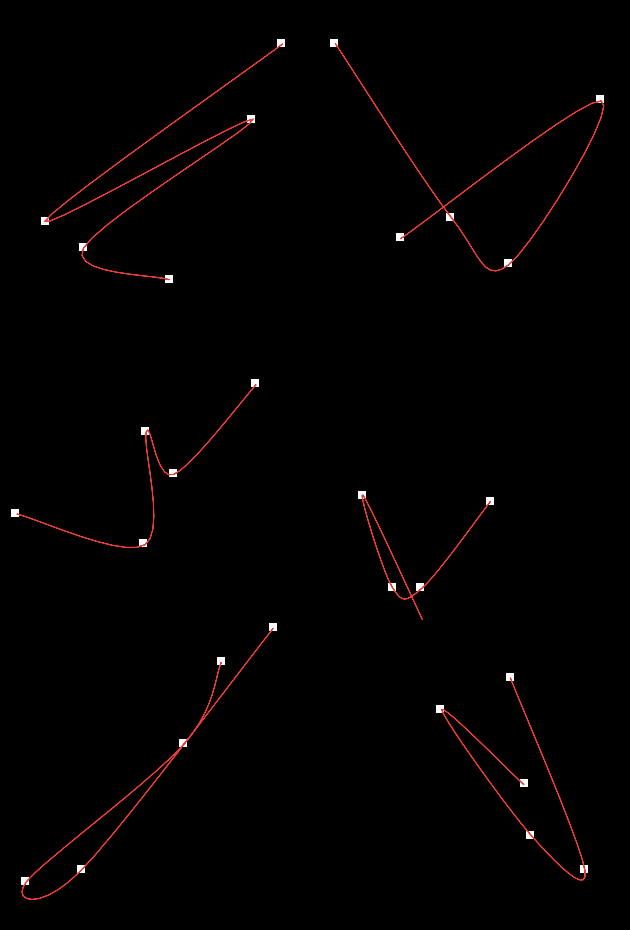
The first tuple we’re drawing in this example will appear as a small white square centered at each input control point. The second tuple will draw a polygon through our interpolated points, but by joining them with their reverse ({x,|x}) this polygon will look like a plain line. Curvature of the line is achieved purely by drawing multiple straight segments.
t: {3(x*)\1}(!11)%10                          / tween [0,1] to the powers [0,3]
c: .5*(0 2 0 0;-1 0 1 0;2 -5 4 -1;-1 3 -3 1)  / catmull-rom coefficients
i: +/t*c(+/*)\:                               / interpolate
s: ,/(+i'+:)'4':{(,*x),x,,*|x}@               / points -> splined points

p: w*0N 2#?10                                 / 5 random points on screen
((_p-2;;4 4#1);({x,|x}s p;,"red"))            / (control points;splined line)
On each run, iKe generates a new set of points and renders a curve:

Experiment with these building blocks and see what kinds of sketches you can come up with- the sky’s the limit.
