When the Macintosh was released in 1984, it featured a square-pixeled black-and-white display at a crisp 72 dots per inch. The 512x342 resolution might seem less than impressive today, but for the time it was a pleasantly high-resolution consumer-grade computer. Among other things, the monospaced Monaco 9pt bitmap font featured characters that were 6 pixels wide, allowing the Macintosh to render a standard 80-column terminal with ample room for a vertical scrollbar and other niceties.
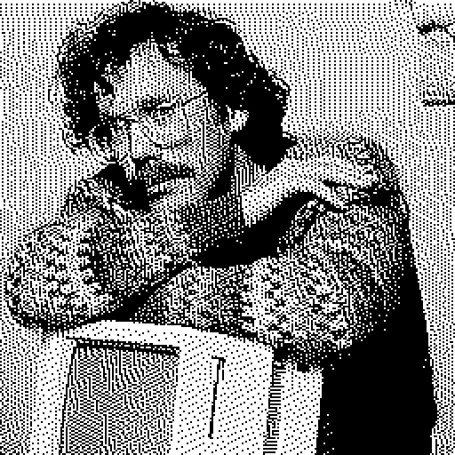
Beyond Susan Kare’s brilliant type design and pixel-art icons, a cornerstone of the visual vocabulary of the Macintosh is the use of dithered images. Dithering algorithms use a small palette (in our case, black and white) to represent a larger one (simulated grayscale). Here we will examine two popular techniques: Floyd-Steinberg dithering, and a variation common on the Macintosh, Atkinson dithering.
The central idea of Floyd-Steinberg dithering is error diffusion. When determining the 1-bit color to assign to a given pixel in a grayscale image, quantizing will result in some error- a pixel either darker or lighter than the true grayscale value. By “pushing” this rounding error to neighboring pixels, we can ensure that on average the distribution of black and white in the output image resembles the input. Your eye closes the gap, and reconstructs some of the lost information.
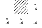
Floyd-Steinberg dithering scans input pixels in a single pass, top-to-bottom and left-to-right. Error left over from each pixel is distributed between neighboring pixels which have not been converted yet, in the following proportions:
Suppose we have the [0.0,1.0] grayscale values of an image in an array pixels and the width of the image w, and we wish to generate an array of {0,1} output pixels. If we are permitted to mutate pixels in-place, a JavaScript implementation of the algorithm might look something like the following:
function floyd(pixels,w) {
	const m=[[1,7],[w-1,3],[w,5],[w+1,1]]
	for (let i=0; i<pixels.length; i++) {
		const x=pixels[i], col=x>.5, err=(x-col)/16
		m.forEach(([x,y]) => i+x<pixels.length && (pixels[i+x]+=err*y))
		pixels[i]=col
	}
	return pixels
}
Given a mask (m) of relative offsets to neighbor pixels and the proportion of error they should get, we map over our pixels in order. The color at each pixel (col) is a simple quantization of the grayscale value (x>.5), the error (err) is the difference between this quantized value and the original, and we simply add a fraction of that error to neighbor pixels before returning col.

Note that in this implementation error diffused from the right edge of the image will bleed into the left edge of the following row. The inherent noisyness of dithering makes this aesthetically irrelevant, and doing so simplifies the implementation. Everyone wins!
If we wanted to avoid modifying pixels in-place, we could observe that the accumulated error we care about would fit in a fixed-size circular buffer (e) proportional to the width of our image. The result is slightly more complex, but in some ways conceptually cleaner, since our main loop is now a map():
function floyd2(pixels,w) {
	const e=Array(w+1).fill(0), m=[[0,7],[w-2,3],[w-1,5],[w,1]]
	return pixels.map(x => {
		const pix=x+(e.push(0),e.shift()), col=pix>.5, err=(pix-col)/16
		m.forEach(([x,y]) => e[x]+=err*y)
		return col
	})
}
(Array.shift() and Array.push() are used here for conciseness; use your imagination for a more efficient low-level implementation.)
Apple’s Bill Atkinson developed a variation of the above technique which produces results that are subjectively nicer-looking. The basics work the same, but error is spread in a broader pattern, and only 3/4ths of the error is preserved:
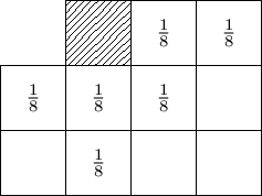
Modifying floyd2() above, we can simplify m, as all the error is propagated in an even proportion. The sliding error window e now needs to be roughly twice as large to account for the broader spread pattern:
function atkinson(pixels,w) {
	const e=Array(2*w).fill(0), m=[0,1,w-2,w-1,w,2*w-1]
	return pixels.map(x => {
		const pix=x+(e.push(0),e.shift()), col=pix>.5, err=(pix-col)/8
		m.forEach(x => e[x]+=err)
		return col
	})
}
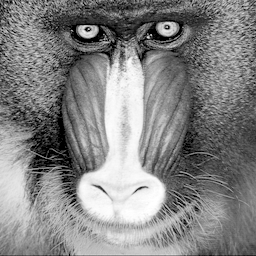


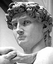
Compared side-by-side with Floyd-Steinberg dithering, Atkinson’s algorithm seems to produce richer contrast, at the cost of some detail in very light or dark areas of the image.
Readers of this blog might be curious to know what Atkinson dithering would look like in iKe.
We can leverage iKe’s capabilities for loading remote images via the special /i operative. By specifying the built-in palette gray, the input image will be converted into a matrix of [0,255] grayscale values. To resize the iKe graphics window to match the image, we initialize the magic variables w and h based on the dimensions of this matrix. Our running error window is stored in a global (e) initialized with two rows worth of zeroes (&2*w). The definition of our mask m is virtually identical to the JavaScript version above.
Most of the work happens in d, which is meant to dither one pixel. We find the value of the current pixel, incorporating accumulated error (p:x+*e), quantize the output color (c:p>.5), shift out the consumed error value and shift in a zero (e::1_e,0), and then amend e by adding the error at the current pixel at every index in our mask m (@[`e;m;+;(p-c)%8]).
To dither the entire image, we explicitly apply d to each pixel of the matrix, remembering to first rescale the input [0,255] palette indices into floating point [0.0,1.0] values. For an animated application of this code, it would be necessary to reset e after each frame.
/i pixels;gray;https://i.imgur.com/Lcq4Xi4.png
w: #*pixels
h: #pixels
e: &2*w
m: (0;1;w-2;w-1;w;2*w-1)
d: {p:x+*e; c:p>.5; e::1_e,0; @[`e;m;+;(p-c)%8]; c}
,(;;d''pixels%255)